Approximate equidistant curve for polynomials
May 02, 2017
13 mins read
Introduction
It is required to have an equidistant curve for a given polynomial for a great variety of applications. For example, an equidistant is needed for a lane detection visual system of a Self-Driving car in case only one line is well determined (the other one is the equidistant because lane lines are parallel). There is an exact solution for the problem and it is known that an equidistant for a polynomial function is a higher order polynomial function.
However, it is usually needed to have an equidistant polynomial of the same order to the given one. For instance, it is essential for the mentioned above application to make the visual system robust and stable. Therefore, an approximate method was developed.
Task: Given the reference polynomial coefficients pol and desired distance d defined perpendicular to the given line, find approximate equidistant line as polynomial of the same degree and return its coefficients pol_eq.
Ideas
-
Create a set of
Npoints with the same orthogonal distance (d)from a given polynomial. -
Fit a new polynomial of desired degree to the point set.
The following simple expressions are useful for the calculations:
Equation of a straight line:
\[y=kx + b;\]To find the slope of a line perpendicular to this line, it is needed to flip the slope coefficient and change its sign:
\[K_m = -1/k;\]Implementation
The implementation will use Python with Numpy and Matplotlib library for results visualisation.
First of all, points correspond to the given polynomial should be calculated. X coordinates of reference points initialized as equally spaced points between 0 and max_l.
# Calculate a polinomial value in a given point x
def pol_calc(pol, x):
    pol_f = np.poly1d(pol)
    return(pol_f(x))

EQUID_POINTS = 20 # N
# pol - given polinimial coefficients (e.q. pol = np.array([-1.0, 2.5]))
x_pol = np.linspace(0, max_l, num=EQUID_POINTS)
y_pol = pol_calc(pol, x_pol)
In order to make things simpler with bounds points and better define the slope coefficients we will consider points in between to neighbour pairs of generated ones. They can be obtained by linear interpolation.
Here we calculate coordinates of such points and direction of perpendiculars as slopes of perpendicular lines (k_m calculated as \( K_m = -1/k \) ), which start from the middle points:
# Calculate polints position between given points
for i in range(len(x_pol)-1):
    y_m.append((y_pol[i+1] - y_pol[i]) / 2.0 + y_pol[i])
    x_m.append((x_pol[i+1] - x_pol[i]) / 2.0 + x_pol[i])
    # Slope of perpendicular lines
    if y_pol[i+1] == y_pol[i]: #Avoid division by 0
        k_m.append(1e8) # A vary big number
    else:
        k_m.append(-(x_pol[i+1] - x_pol[i])/(y_pol[i+1] - y_pol[i])) # Slope of perpendicular lines
Shifts dx and dy of the equidistant points (x_eq and y_eq) from the middle reference points (x_m and y_m) should be calculated. In fact, dx = x_eq - x_m and dy = y_eq - y_m.
Taking into account the Pythagorean theorem:
\[dx^2 + dy^2 = d^2;\]And \( K_m \) definition: \( K_m = \frac{dy}{dx}; \)
One can found out dx and dy:
Here the calculations implemented with respect to desired position (sign of d) of the equidistant and the reference points positions.
#Calculate equidistant points
x_eq = d*np.sqrt(1.0/(1 + k_m**2)) # Calculate reference shift of the equidistant points
y_eq = np.zeros_like(x_eq) # Create np.array for y_eq
if d >= 0: # x positions of the equidistant depends on direction
    for i in range(len(y_m)):
        if k_m[i] < 0:
            x_eq[i] = x_m[i] - abs(x_eq[i])
        else:
            x_eq[i] = x_m[i] + abs(x_eq[i])
        y_eq[i] = (y_m[i] - k_m[i] * x_m[i]) + k_m[i] * x_eq[i]
else:
    for i in range(len(x_m)):
        if k_m[i] < 0:
            x_eq[i] = x_m[i] + abs(x_eq[i])
        else:
            x_eq[i] = x_m[i] - abs(x_eq[i])
        y_eq[i] = (y_m[i] - k_m[i]*x_m[i]) + k_m[i] * x_eq[i]
The final step is to fit a new polynomial of desired degree to the point set
pol_eq = np.polyfit(x_eq, y_eq, len(pol)-1)Results and discussion
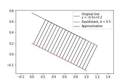
As a result, the algorithm is able to produce reasonably well defined equidistant in a simple linear case:
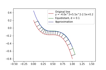
As well as in case of higher order polynomial:
However, in case of real application, one should keep in mind two notes:
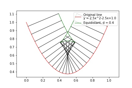
- Equidistant is not always a smooth function because of geometrical restrains:
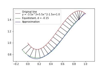
- The algorithm use the same
xcoordinates of points for reference points set and for building approximation. That is why it is forced to “predict” the reference line behavior in an extended interval. It can lead to unexpected results, especially in case of high order polynomial:
The last issue can be addressed by wise extending x range of the reference points set.
The code
Final code of the project with visualisation.
import numpy as np
import matplotlib.pyplot as plt

# Calculate a polinomial value in a given point x
def pol_calc(pol, x):
    pol_f = np.poly1d(pol)
    return(pol_f(x))

# Create original line text equation for a plot legend
def text_eq(pol):
    str_eq = 'Original line\ny = '
    j = 1
    for i,p in enumerate(pol):
        print(p)
        str_eq += str(p)
        order = len(pol) - j
        if order > 1:
            str_eq += ('x^'+str(order))
            if pol[i+1] > 0:
                str_eq += '+'
        elif order > 0:
            str_eq += ('x')
            if pol[i+1] > 0:
                str_eq += '+'
        j += 1
    return str_eq

#Calculate approximated equidistant to a parabola
EQUID_POINTS = 20 # Number of points to use for the equidistant approximation

def equidistant(pol, d, max_l = 1, plot = False):
    x_pol = np.linspace(0, max_l, num=EQUID_POINTS) # Reference curve points
    y_pol = pol_calc(pol, x_pol)
    x_m = [] # Mid points
    y_m = []
    k_m = []
    # Calculate polints position between given points
    for i in range(len(x_pol) - 1):
        y_m.append((y_pol[i+1] - y_pol[i]) / 2.0 + y_pol[i])
        x_m.append((x_pol[i+1] - x_pol[i]) / 2.0 + x_pol[i])
        # Slope of perpendicular lines
        if y_pol[i+1] == y_pol[i]: #Avoid division by 0
            k_m.append(1e8) # A vary big number
        else:
            k_m.append(-(x_pol[i+1] - x_pol[i])/(y_pol[i+1] - y_pol[i])) # Slope of a perpendicular
    # Convert arrays into np.arrays
    x_m = np.array(x_m)
    y_m = np.array(y_m)
    k_m = np.array(k_m)
    # Calculate equidistant points
    x_eq = d*np.sqrt(1.0/(1 + k_m**2)) # Calculate reference shift dx of the equidistant points
    y_eq = np.zeros_like(x_eq) # Create np.array for y_eq
    if d >= 0: # x positions of the equidistant depends on direction
        for i in range(len(y_m)):
            if k_m[i] < 0:
                x_eq[i] = x_m[i] - abs(x_eq[i])
            else:
                x_eq[i] = x_m[i] + abs(x_eq[i])
            y_eq[i] = (y_m[i] - k_m[i] * x_m[i]) + k_m[i] * x_eq[i]
    else:
        for i in range(len(y_m)):
            if k_m[i] < 0:
                x_eq[i] = x_m[i] + abs(x_eq[i])
            else:
                x_eq[i] = x_m[i] - abs(x_eq[i])
            y_eq[i] = (y_m[i] - k_m[i] * x_m[i]) + k_m[i] * x_eq[i]
    # Fit a polinomial of order which is the same to the given one to the equidistant points
    pol_eq = np.polyfit(x_eq, y_eq, len(pol) - 1)
    # Visualize results
    if plot:
        # Original line
        plt.plot(x_pol, y_pol, color='red', linewidth=1, label = text_eq(pol))
        # Equidistant
        plt.plot(x_eq, y_eq, color='green', linewidth=1, label = 'Equidistant, d = '+ str(d))
        #Approximation
        plt.plot(x_pol, pol_calc(pol_eq, x_pol), color='blue',
                 linewidth=1, label = 'Approximation')
        plt.legend() # Add legend
        plt.axis('equal')
        # Draw black connection lines
        for i in range(len(x_m)):
            plt.plot([x_m[i], x_eq[i]], [y_m[i], y_eq[i]], color='black', linewidth=1)
        plt.show()
        #plt.savefig('./equid.jpg')
    return pol_eq

# Use example
pol = np.array([-4.0, 5.5, -2.5, 0.2])
print(equidistant(pol, -0.1, plot=True))
The code was used in the Lane Lines Detection project.