Adaptive Virtual Sensors for Lane detection

Introduction

One may use different approaches based on combination of threshold filters for defining pixels on an image, which represent the lane line. However, it can be quite challenging because the lighting conditions may vary even in one video frame from the front facing camera due to shadows appearing and etc. That is why, an adaptive approach with virtual sensors is proposed here.

Key ideas

• Image can be analyzed with Adaptive Virtual Sensors. Each sensor is a string of pixels (for example, 30 pixels long) in the area where it is expected to find a line. Virtual sensor can find the line position or can find nothing. The point with the maximum value (brightness) in the virtual sensor is a suspected line point. Line point considered found if its value minus the mean pixels value of the sensor is larger than the threshold and the point is shifted from the sensers center on less than DEV pixels.

• Image is analyzed from the bottom to the top because it is the most probable to find a line on the closest to the car road pixels because resolution is higher near to the hood. Position of the next sensor is predicted by position of the previous line point (in case of a still image) position or calculated from the polinomial fit of points which were found on the previous frame (in case of a video).

• Threshold value should be selected independently for each virtual sensor based on mean value of pixels in the sensor. In general, the threshold should be as large as possible to reduce false positive results. But in the bright areas it should be less because the region marred by the sunlight and line contrast decreased. It should also be less for the dark areas, as the line is poorly distinguishable in the dark. It allows to find line points on an image with both deep shadows and bright areas which is very challenging in case of using a constant threshold for the whole image.

• Polynomial fit on the set of points, found by virtual sensors, is then applied. The best order of the polynomial should be chosen for each points set individually.

• If only one line is visible, then the second can be carried out as an equidistant at road width distance from the first one.

Order of a polynomial

One of the key ideas of the project is the usage of the reasonable minimal order of polinomial functions for lines fitting (order should be in range [1,3]). The function best_pol_ord chooses such order. It starts from a linear function and, if it does not perform well enough, increases the polinomial order (up to 3). It returns polinomial coefficients and mean squared error of the selected approximation. The function stops increasing the order if it does not help (mean squared error drops not significant in case of higher order) or in case the mean squared error is small enough (< DEV_POL).

import numpy as np
from sklearn.metrics import mean_squared_error

DEV_POL = 2 # Max mean squared error of the approximation
MSE_DEV = 1.1 # Minimum mean squared error ratio to consider higher order of the polynomial
def best_pol_ord(x, y):
    pol1 = np.polyfit(y, x, 1)
    pred1 = pol_calc(pol1, y)
    mse1 = mean_squared_error(x, pred1)
    if mse1 < DEV_POL:
        return pol1, mse1
    pol2 = np.polyfit(y, x, 2)
    pred2 = pol_calc(pol2, y)
    mse2 = mean_squared_error(x, pred2)
    if mse2 < DEV_POL or mse1 / mse2 < MSE_DEV:
            return pol2, mse2
    else:
        pol3 = np.polyfit(y, x, 3)
        pred3 = pol_calc(pol3, y)
        mse3 = mean_squared_error(x, pred3)
        if mse2 / mse3 < MSE_DEV:
            return pol2, mse2
        else:
            return pol3, mse3

It is possible to use a simple low pass filter or an alpha-beta filter for smoothing polynomial coefficients of the same degree. But for two polynomial with different orders a dedicated function smooth_dif_ord can be introduced. It calculates average x position of points for a given function f(y) at y values from the new dataset and fit these new average points with polinomial of desired degree.

# Smooth polinomial functions of different degrees   
def smooth_dif_ord(pol_p, x, y, new_ord):
    x_p = pol_calc(pol_p, y)
    x_new = (x + x_p) / 2.0
    return np.polyfit(y, x_new, new_ord)

The pipeline demonstration

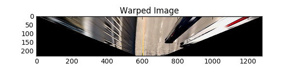
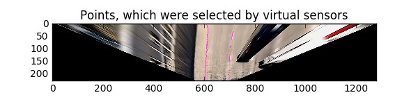
After image warping the algorithm perform points finding by the described above in the Key ideas section points finding approach. Basically, virtual sensors are filters with an adaptive region-of-interest and adaptive threshold.

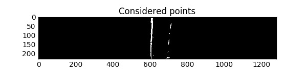
Each virtual sensor considers points which have values higher than mean pixel value in the sensor plus the threshold value (it is a kind of local binary image for the virtual sensor). The threshold value is calculated for each sensor individually based on the mean value of pixels in the sensor. The line point is the pixel with the maximum value among all considered pixels. The sensor position (ROI) determinated by the position of the previously detected line point (for still images) or by the polynomial fit of line points from the previous frame (for videos).

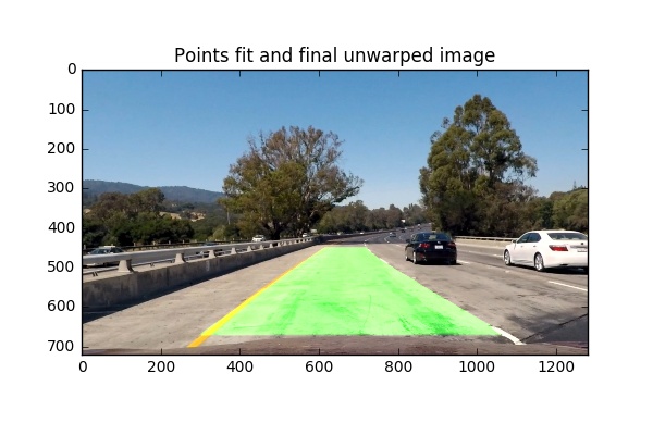
Code of the discussed approach is availuabe on Github in the project repo.