Semantic Segmentation of Seismic Reflection Images

This post contains a description of the 14th place solution by Argus team (Ruslan Baikulov, Nikolay Falaleev) of the TGS Salt Identification Challenge. For the challenge overview, see another post.

Hard- and software

The main deep-learning framework of the solution is PyTorch 0.4.1, which is well known for its flexibility and simplicity. Previously developed open source framework Argus simplifies the experiments with different architectures and allows to focus on deep learning trials rather than coding neural networks training and testing scripts. We also use OpenCV to solve computer vision-related tasks during pre- and post-processing stages. Despite the fact that the main code is written in Python, the puzzle-solving part is based on R code, because this programming language used as the primary language of the original algorithm author. Solution code for experiments and submission encapsulated into an nvidia-docker container for portability.

Our main GPU computational power used for the competition consists of:

 1x RTX 2080 Ti
 3x GTX 1080 Ti
 1x GTX 1070

See the GPU’s performance compare here.

The GPUs are distributed among several PCs. However, in some cases, some extra cloud-based instances with Nvidia V100 were utilized, when it was reasonable to increase calculations on graphical cards extensively. Particularly, they were used when it was necessary to train many folds for cross-validation or to conduct serial experiments. Although a lot of GPUs were used during experiments, the final models can be trained in about one week on a single GTX 1070.

Puzzle-solving fun

It was found out that the provided tiles combine into several mosaics if pieces from both subsets: training and testing are used. This information potentially can gain training results. However, a large number of pieces and brightness difference of neighbour tiles make the assembly task rather difficult. It should also be mentioned, that total number of original mosaics and their shapes are not known. One contestant (Vicens Gaitan) of the Challenge provided an outstanding public kernel for mosaics assembling. The main idea of the program is to find thresholded nearest neighbours for tiles in four directions with a kNN algorithm. The similarity of tiles sides estimated by a mean similarity of linear pixel value extrapolation for boundary pixels. See the public Kernel for details.

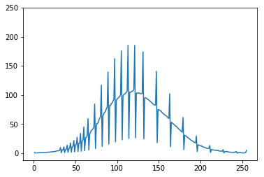
Mean histogram of images. Spikes may be introduced during preparation steps by the organizers.

We used the code as is, without significant modification. However, one trick was applied to overcome brightness difference of neighbouring tiles. It looks like each picture was undergone histogram normalization in such a way that resulted in the most bright pixel to be at 255 level and the darkest - 0. This resulted in a brightness shift. So, histogram matching to the average histogram can help to equalize tiles and make the neighbour pieces more similar. Actually, this helps to merge more pieces into mosaics (>6000, including mosaics with two and more pictures).

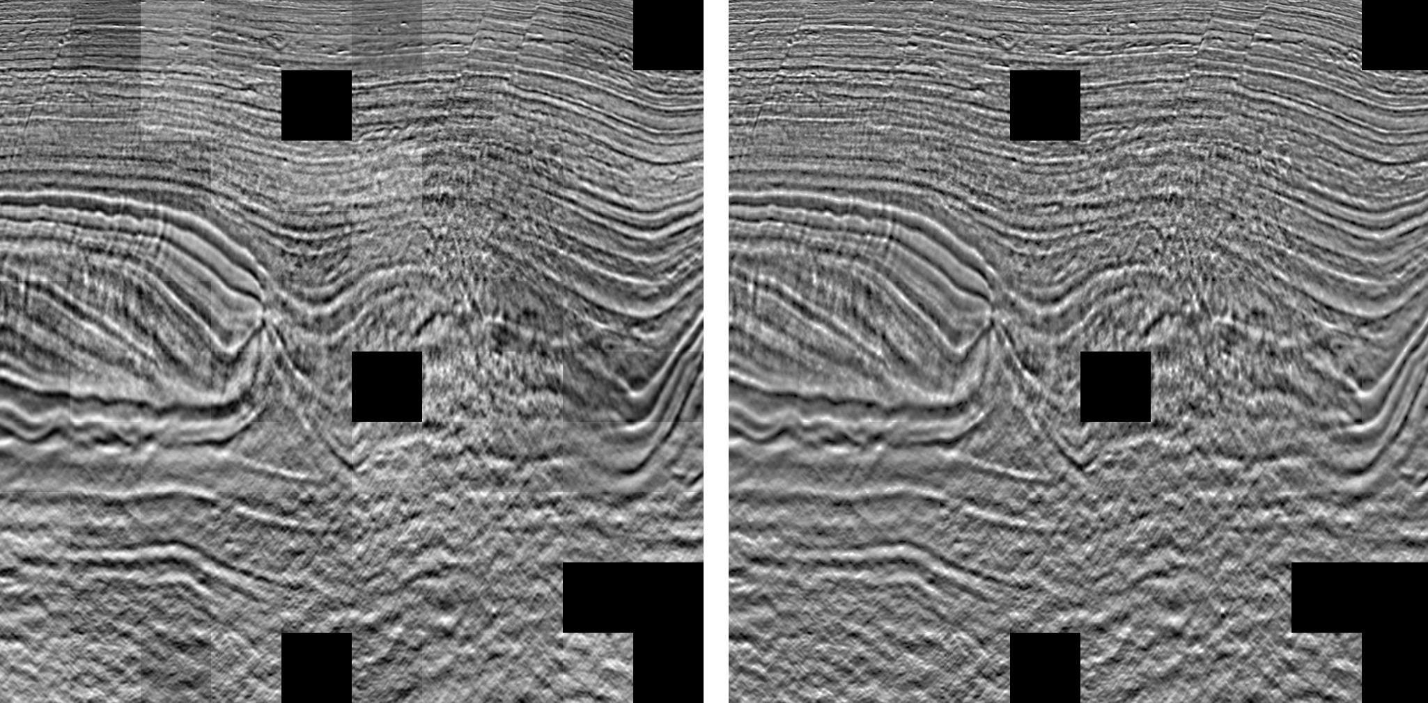
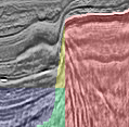
A mosaic before (left) and after (right) histogram matching, which eliminates visual inconsistency of brightness between tiles.

Also, two great Python implementations of jigsaw puzzle problem were tested. The code looks promising on small subsets of images but requires an enormous amount of time on the whole dataset, and the calculation was not completed.

An interesting detail was observed after puzzles assembly. It looks like top salt/sedimentary interface was the only actual markup with straight vertical lines as side boundaries while interior pieces of the salt dome (pieces without any boundaries) labeled as empty. This confused neural networks as textures inside salt domes are pretty different from textures outside of salt areas.

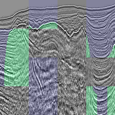
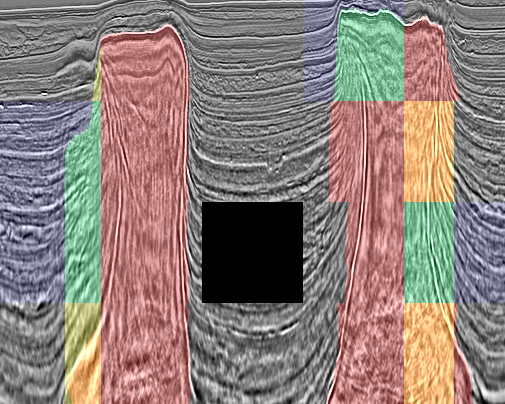
No salt labeled inside a salt dome. Green - salt areas as marked in the train dataset; blue areas - pixels marked as empty. Patches without any labels are from the test subset.

Data preprocessing

Most Convolutional neural networks for semantic segmentation require input tensor size multiple of 32. Hence, the original images with size 101x101 should be padded. The most straightforward approach of zero (or constant) padding was tested on pair with a reflection padding. The latter worked satisfactorily. However, it was found out that it is better to pad images to the required input size with biharmonic inpaint from skimage package. This led to a score improvement for the most of used models. We also tried to inpaint only missed parts of mosaics. However, it was not a successful experiment in both cases. The first one uses raw tiles, and this confuses CNNs as they have to see neighbouring tiles with random brightness. The second uses images after histogram match, and, obviously, such data process lost some useful information and this results in a lower metric.

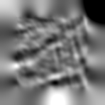An inpainted to 148x148 px sample.

Different approaches to data augmentation were examined. However, most of them didn’t help due to the nature of the samples (for instance, there is no sense to flip images in up-down direction). Finally, original images were inpainted to 148x148 px and sampled with the random crop to the input size 128x128 px. Flip in the left-right direction and random linear color augmentation (for brightness and contrast adjustment) were applied during the data augmentation step.

Models

Most recent deep learning architectures for semantic segmentation are based on an encoder-decoder structure with so-called skip-connections. Two types of architectures were involved in experiments: U-Net and LinkNet style. Surprisingly, in most cases U-Nets outperforms more modern LinkNets. These architectures were tested with different encoder blocks. All in all, the following encoders were subjected to experiments:

ResNet(18, 34, 50, 101, 152)
DPN92
SE-ResNeXt(50, 101)
SENet154
DenseNet161

Interestingly, heavier encoders performed better in most cases, despite an obvious lack of training data.

Dropout layers were introduced into network architectures in order to reduce overfitting. Dropout layers were situated not only in between decoder blocks but in skip connections as well.

Two different upsampling layers can be used as decoder blocks: with a transposed convolutions and a traditional upsampling. In addition to a normal decoder branch, we add an FPN-style decoder. The optimal number of layers in the part was developed after several attempts.

In addition to the segmentation task, an additional branch was added into basic network architecture for images classification on two classes: empty/contains salt. It consisted of several fully connected layers after a global average pooling. The branch utilized bottleneck feature map as input and was trained along with the primary task training with a BCE loss function. All tiles, classified as empty, were filled with zeros on the prediction step.

The first max-pool layer was excluded from all encoders as it helps to increase the spatial resolution of predictions and, consequently, get the score better.

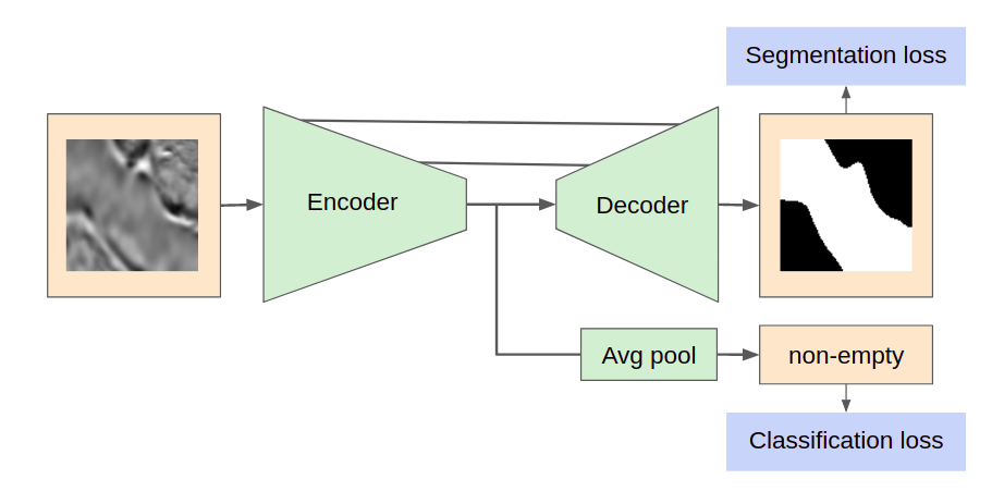General scheme of the neural networks architectures.

For details of the networks implementations, please, check out the GitHub repo.

Approaches to training

The training process looks like the following after hyperparameters optimization by manual try-and-error process with some support by an automated grid search.

• Loss: Lovasz hinge loss with elu + 1. See details here
• Optimizer: SGD with LR 0.01, momentum 0.9, weight_decay 0.0001
• Train stages:

a. EarlyStopping with patience 100; ReduceLROnPlateau with patience=30, factor=0.64, min_lr=1e-8; Lovasz * 0.75 + BCE empty * 0.25

b. Cosine annealing learning rate: 300 epochs, 50 per cycle; Lovasz * 0.5 + BCE empty * 0.5

Post-processing - one of the keys

The evaluation metric assessed checkpoints and the best one was taken for the final prediction for each fold. The arithmetical mean of prediction, made by all models, was binarized by thresholding. The binary images were subjected to further processing.

Given we have a lot of test images assembled into mosaics, tiles interaction should be taken into account. The below techniques are not relevant to the real-world task, but help to improve the competition score. It is worth saying that the use of such approaches can be justified by the fact that the real task has another data as compared with the data in the competition and do not have to deal with mosaics of the kind at all.

The evaluation metric penalize quite hard missing of masks even if it has an area of several pixels. So, there were several cases of missed small masks corners. To fix this issue, a heuristic was introduced. It detects such cases and connects already presented masks with a third order polynomial. Boundary conditions of the smooth first derivative were applied.

A missed corner of a salt body restorated by the post-processing algorithm. Green/blue - salt/empty regions from the train dataset, red - predicted mask, yellow - inpainted by the post-processing.

We automatically copied train tiles with vertical lines markup down the mosaic. We also copied it upward to the terminal level of tiles. The level was defined as the level with a predicted mask which has two or more times less “salt” pixels on the top edge as compared with the bottom one. In case there is no such tile in the tile column, the level is defined as the top level of such tiles among other tile columns in the considered mosaic. We also set to zero all predicted masks below tiles with all “salt” pixels on the bottom edge in order to exclude all positive salt segmentation from inside the salt domes.

Example of the whole mosaic post-processing. Green/blue - salt/empty regions from the train dataset; red - predicted mask; yellow - inpainted by the post-processing (used in the final submission).

Due to the data nature, holes inside masks makes no sense, so, a dedicated loop fill all detected holes in the predicted masks.

Final results

Pipeline of the best submission

• Inpaint images and masks to 148x148 px
• Train with augmentations: random crop 128x128, random horizontal flip, random linear transform of color.
• Average of two training processes:
  • SE-ResNeXt50 on 5 random folds.
  • SE-ResNeXt50 on 6 mosaic based folds (similar mosaics tiles placed in the same fold) without the second training stage.
• Thresholding 0.4 for segmentation and 0.5 for empty/non-empty.
• Postprocessing

Unsuccessful ideas

Many other approaches and algorithms were tested but didn’t result in local validation score improvement, that is why they were not used in the final submission pipeline.

• All kind of augmentations, except horizontal flip and random linear color transform (brightness and contrast adjustment). There was lack of improvement while random Gaussian noise was applied as well as speckle noise, which was especially surprising. It seems strange because in most tasks associated with real-world physical measurements such augmentations work quite well as they correspond to natural measurement processes errors. From our perspective, the observation may be explained by the nature of the provided data, which was processed by the challenge hosts. And the processing made described noise augmentation models irrelevant.
• Training on patches with available parts of mosaics.
• Inpaint two random tiles. We tried to inpaint in gaps between several random input images to simplify the process and make results more natural as the inpainting algorithm has references on both edges.
• Different LR for backbone and decoder parts of the neural network architecture. We tried to reduce LR for backbone as we use pretrained encoders. However, it did not help.
• CoordConv as extra input channels.
• CUnet, which is stacked U-Nets with U-Net block coupling. The architecture may produce great results, however, in the case, lack of data led to overfitting.
• Mean Teacher. Have a gain with a small ResNet34 encoder, but not with large.
• Any attempts to make use of depth data. We tried to concatenate depth to the input image as an extra channel, filled with the same value and feed depth directly into the CNN bottleneck without any success.

Untested ideas

In addition to discussed above ideas, several promising approaches were not examined. Here it is a list with some of them.

• Pseudo labeling. According to other participants, this technique may be quite useful. Given the puzzles are known to some extent, one may wisely choose only tiles with the salt edge to add into training or introduce other heuristics which may help to subset only reliably marked samples. Some samples may also be post-processed before adding to the training dataset as described above. However, one should use the technique with caution as it is effortless to overfit to the public leaderboard.
• A more advanced step-by-step training approach, such as Data Distillation.

Conclusions

Our team managed to finish on the 14th place out of 3234 competing teams. The results are based on a step-by-step improvement of the pipeline, postprocessing, and fair cross-validation. Finally, results were achieved by carefully selected architectures without heavy ensembles of neural nets and second order models. Reasonable cross-validation with the evaluation metric prevented us from overfitting on the public leaderboard.

Acknowledgments

We would like to thank our friends and families for supporting us during the Challenge.

We appreciate that two GPUs GTX 1080 Ti were provided for experiments by our employer, Constanta.

The project code is available on Github.