Top-1 solution of SoccerNet Camera Calibration Challenge 2023

SoccerNet Camera Calibration Challenge 2023 Task

This technical write-up describes some details of the winning submission to the SoccerNet Camera Calibration Challenge 2023, one of the challenges held at CVPR 2023.

The objective of the challenge in 2023 was to generate precise camera calibration values, including intrinsic parameters for the pinhole camera model as well as extrinsic parameters, using individual frames extracted from football broadcast videos.

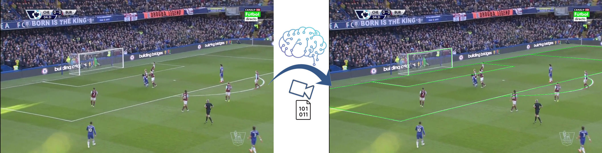Fig. 1. An original input video frame and a football pitch model overlay (represented by green lines) drawn using the predicted camera calibration values.

The predicted camera parameter’s quality was assessed by measuring their ability to accurately reproject the football pitch model onto the image. This evaluation process formulated the camera parameters evaluation as a binary classification problem: the projection of a line or a circle was considered correct if all its extremities (or all points annotated for circles) had a reprojection error lower than 5 pixels (denoted as \( Acc@5 \)). Additionally, the resulting accuracy was multiplied by a completeness factor, representing the fraction of images for which predictions were provided. Thus, the final combined metric can be expressed as \( Metric = Completeness \times Acc@5 \).

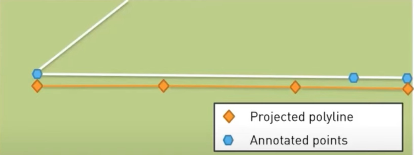Fig. 2. The accuracy metric. Image is from the official presentation.

In total, there were 16463 images in train subset, 3212 in validation subset, 3141 in test subset, which was used for public leaderboard results and was accompanied with annotations and 2690 images in the challenge subset without annotations, the subset was used for the final leaderboard results. All images have 960x540 px resolution.

Annotation classes contained 23 lines (each line represented as two or more points) and 3 circles (represented by sets of points).

More details on the challenge metric and the challenge itself can be found in the official repo.

The project code is available on Github.

The solution ideas

An accurate pitch model is available, providing real-world coordinates of various keypoints on the pitch, such as line intersections, penalty points, the pitch center, and etc. Furthermore, the pitch model allows calculating coordinates of numerous additional points on the pitch. This implies that it is feasible to leverage the pitch model coordinates with corresponding points detected in the images to conduct standard camera calibration, just using the pitch model instead of a traditional checkerboard calibration pattern.

In total, the solution used 57 keypoints.

Intersections

The provided data annotation contained manually annotated points on the lines. However, in many cases, the provided data lacked accuratre intersection points of the lines, which were crucial for calibration purposes, considering the intersection coordinates of lines in the pitch model. To address this limitation of the annotation, 30 points were defined as the intersections of linear data fitting applied to the line points provided in the annotation. This approach not only enabled the generation of accurate intersection points but also facilitated automated filtering of annotated, making it straightforward to exclude outliers and unrealistic intersections.

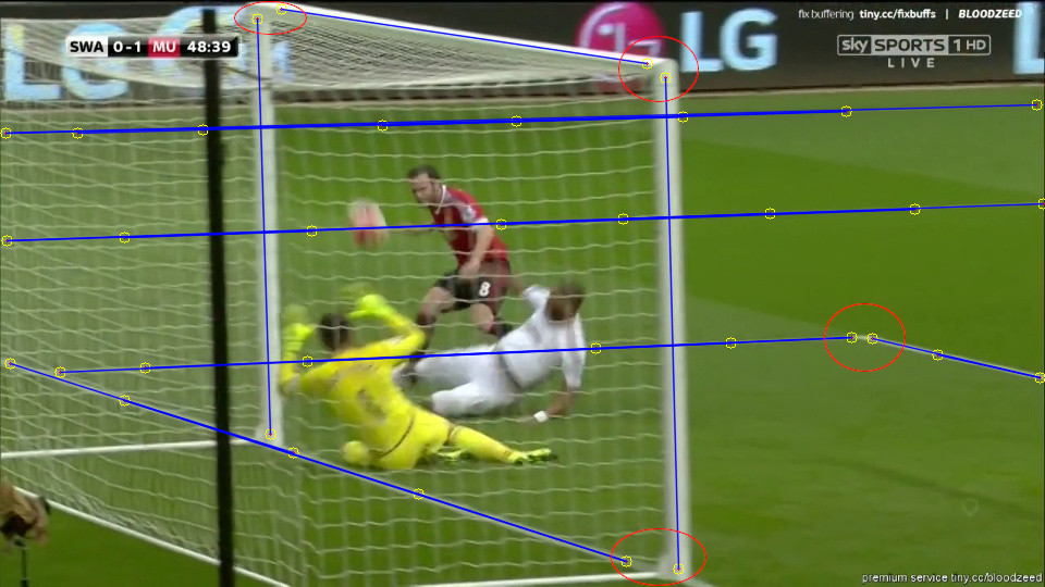Fig. 3. Annotation sample. Small red dots with yellow circles show the points from annotation. As many intersections were not included in annotation, it was nessesary to perform linear fitting of the annotation to find the lines intersections.

Conics intersections

Additional set of 6 points were defined as intersections between conics (’Circle central,’ ’Circle left,’ and ’Circle right’ from the annotation classes) and lines. The conics points from annotation were fitted with ellipses using Halı́ř–Flusser’s ellipse fitting algorithm [1]. For this purpose, the Python package lsq-ellipse was utilized, as it provides a reliable implementation of the algorithm. The intersections were derived analytically as points of ellipse-line intersection.

Tangent points

In many cases, there were still insufficient intersections to construct a homography (<4), while circles are present. Therefore, a correspondence between tangent points of tangent lines from a known point to the circles was utilized to augment the overall number of available points for homography construction. The tangent points were analytically derived using the ellipse equation and the known location of an external point. So, further 8 points were defined as tangent points of tangent lines from a known point to an ellipse.

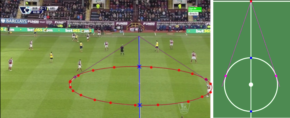Fig. 4. Red dots - circle points from annotation, red curve - the points fitting with an ellipse, blue crosses - ellipse-line intersections, purple crosses - the defined tangent points to the ellipse. There corresponding points on the pitch pattern are shown on the right side.

Additional points

Using the homography created with points from the previous categories, additional 9 points along the central pitch axis (including the pitch center and penalty points) and 4 points to mark quarter turns on the central circle. This approach utilized corresponding real-world points. What is more, the homography allowed including other missing points (e.g., when some lines were not annotated).

Fig. 5. The pitch pattern with all the points depicted. Red - line-line intersection, blue - line-conic intersection, purple - conic tangent point, dark-green - other points projected by homography

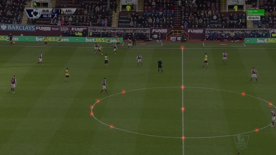Fig. 6. All the points heatmaps target tensor overlayed an input image.

In cases where homography was unavailable due to a limited number of points, the points that should have been marked by homography were masked out in the loss function.

Left-right ambiguity

In scenarios where the camera alignment coincided with the direction of the long axis of the pitch, it became challenging to differentiate between the left and right sides accurately. However, it is crucial to indicate a clear distinction between the two sides in the ground-truth values, particularly when both goals are visible. To address this left-right ambiguity, a remapping process was implemented to ensure consistency. The points were remapped in such a way that the goal area closest to the camera was consistently considered as the left side.

Neural network

The keypoint detection employed the HRNetV2-w48 backbone [2]. To enhance spatial resolution of the predicted heatmaps, we added 2x upsampling and skip-connection features concatenation from the corresponding resolution of the convolution stem. The final predictions had half the resolution of the original image, with softmax used as the last activation. The target tensor consisted of 2D feature maps for each point, where Gaussian peaks \( \sigma = 3 px \) were positioned at the keypoint locations. An extra target channel was included, which represented the inverse of the maximal value among the other target feature maps, ensuring that the final target tensor summed up to 1.0 at each spatial point. Only points within the image boundaries were used as targets.

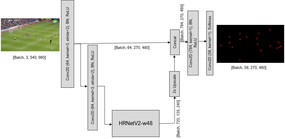Fig. 7. The neural network architecture.

The model was trained using MSE loss and the Adam optimizer. The initial learning rate was 0.001 and was halved when the loss did not improve for 8 consecutive epochs. This halving continued until there was no improvement for 32 epochs. Subsequently, the neural network was finetuned using the Adaptive Wing Loss with the same strategy and starting learning rate of 5e-4. The best checkpoint was selected based on the combined metric value on the valid dataset.

In addition to points detection, there was a line detection neural network, which acts in the same way. Each line of the 23 lines from the annotation was encoded as an individual channel in the target tensor, presenting the heatmap by two Gaussian peaks at the location of the line extremities. The neural network architecture was the same as the previous one but without the upscaling.

Camera calibration

The keypoint set obtained from the points detection model was expanded by including intersections of lines generated by the second model in cases there were not enough points detected on the groundplane by the keypoints model. This augmentation ensured sufficient points for camera calibration, when keypoints within the image were insufficient, as lines intersection points beyond the image boundary were considered, plus, the missing points from the keypoint detection were addressed.

Camera calibration used the calibrateCamera method from OpenCV 4.7, a standard pinhole camera model was utilized without astigmatism and distortions. Despite experiments that involved adding distortions and even using ground-truth values to assess the feasibility of accounting for distortions, the results were consistently lower, possibly due to imperfections in the annotation.

In addition to the points on the ground plane, two additional vertical planes containing the goal polygons were taken into consideration. This increased completeness by providing predictions when there were insufficient points on the ground plane (e.g., in images, depicting the goalposts area only) and improving overall accuracy by incorporating more calibration points (so, not only the points on the ground plane were utilized for this solution, but also the points on the crossbars of the goals).

The camera calibration process was repeated on several subsets of the keypoints, selected by various heuristics:

• all keypoints, thresholded by confidence;
• only keypoints, which correspond to the original line intersections;
• all keypoints after filtering potential outliers using RANSAC homography finding (ground plane points that could not be fitted by the homography reprojection with a 5 px tolerance were excluded in this case) - this heuristic is helpful in situations when the neural network misclassifid some of the points, so the RANSAC filtering will exclude the outliers;
• only the groundplane points, thresholded by confidence;

The final camera calibration values were determined through a heuristic voting process, which considered the root mean square error (RMSE) of the reprojection. The camera parameter set that yielded the lowest RMSE was selected as the final prediction, with preference given to the parameters based on all detected points if the RMSE was <5 px .

To optimize the keypoint detection confidence threshold and the prediction mechanism parameters, Optuna was utilized. The objective was to maximize the combined metric value on the “valid” dataset. Through the optimization process, the parameters were tuned to achieve the best possible performance.

Dataset	Acc@5	Completeness	Metric
Test	76.675	73.425	0.56299
Challenge	73.2247	75.5853	0.55347

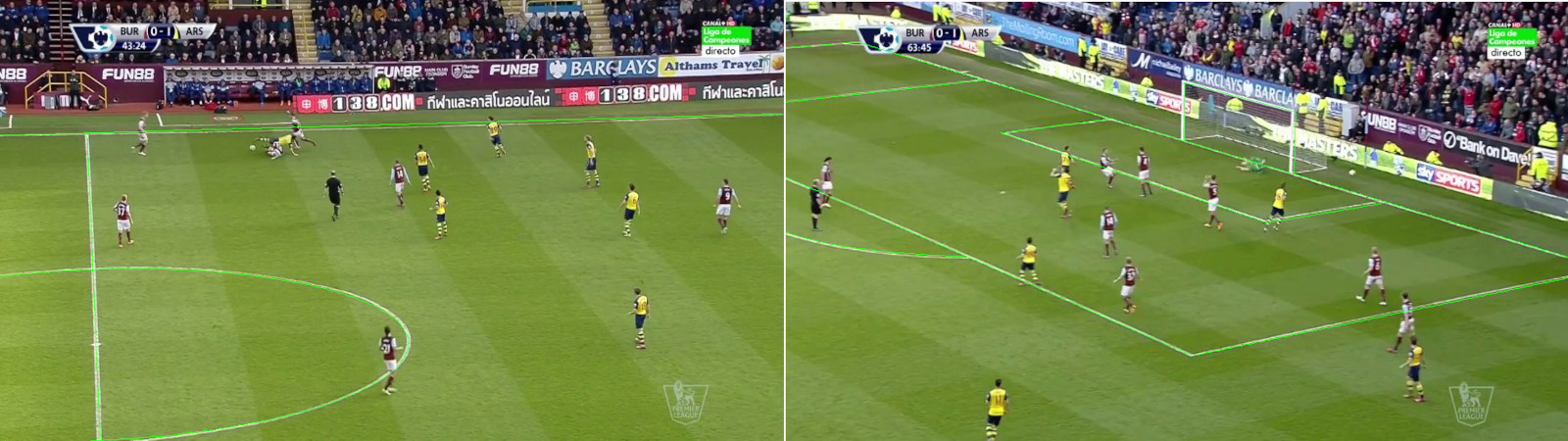Fig. 8. Some results of the camera calibration.

The results appeared to be the best on the challenge leaderboard. Even though the approach cannot be considered general, it or some of the tricks described above can be used for various applications such as online camera calibration or refinement of extrinsic camera parameters, particularly when a well-known pattern is available within the camera’s field of view.

References:

[1]: Radim Halı́ř and Jan Flusser. Numerically stable direct least squares fitting of ellipses. 1998

[2]: Jingdong Wang et al. Deep High-Resolution Representation Learning for Visual Recognition. arXiv:1908.07919